Table of content

A Regression

When we want to make an inference about something we have a tendency to reached for the regression or some of its derivatives, be it linear or non-linear.

In statistics it is often used for its simplicity and powerfulness, as it can be manipulated to fit a trove of different sets of data.

In machine learning it is many times used as a first estimate of the problem you are trying to model, and works in many cases as a benchmark for how good your more sophisticated techniques are.

My purpose of this article is to go through different sorts of regressions, code them from scratch and explain the different results.

To be comfortable following it would be advisable to have some coding experience, does not matter the language as python is quite easy to understand. But I will not delve into specific details of the code.

#Libraries imported
import pandas as pd
import numpy as np
import seaborn as sns
import matplotlib
import matplotlib.pyplot as plt

import scipy.stats as stats
from sklearn.model_selection import GridSearchCV, train_test_split
from sklearn.metrics import mean_absolute_error

%config InlineBackend.figure_format = 'retina' #set 'png' here when working on notebook
%matplotlib inline

Types of regressions

There are several types of regressions, but we will start with OLS, since it is the best linear unbiased estimator (BLUE).

Ordinary Least Square is usually what people mean when they talk about regressions, however, there are several different techniques that are used, such as Weighted Least Square, Generalized Least Square and many more.

But for brevity I will not go through them all, but a mere subset, and then I leave it up to the reader to explore further.

Ordinary Least Square Regression (OLS)

OLS is a subset of the regression family, and is probably the most used technique for solving a regression.

A simple model would be the univariate regression:

$$ y = \beta_{0} + \beta_{1} * x + \epsilon $$

In a linear regression you will have a dependent variable, which is often called the target variable. This is the variable you want to study, to predict or model, and is referred to as: $ y $. The $ x $ represents the independent variable, and as such the variables you use to try to model $ y $.

Example of $ y $ could be how far a car will drive (kilometer), and $ x $ could be the amount of gas in the tank. There is a chance that the distance the car will go has something to do with the amount of gas in the tank.

The second term in the model $ \beta_{1} $ is the parameter which describe how much the variability in $ x $ affects $ y $. So if the independent variable is liters of gas in the tank, and $ \beta_{1} $ is 3, then for every litre extra in the tank, the car will drive 3 kilometer longer.

The first term in the model: $ \beta_{0} $ is the intercept. This describe how far the car will drive if $ x $ is zero, in other words the tank is empty. In this case it is reasonable to believe $ \beta_{0} $ is zero, but mostly the intercept will have an impact on the dependent variable $ y $.

The third term is the $ \epsilon $ which is the error term, and this is the variation in the dependent variable the independent variables fails to capture: $ y - (\beta_{0} - \beta_{1} * x) = \epsilon $. Going back to the car example, the profile of the tires, the efficiency of the engine, the weight of the car and the air pressure in the tires might also have an impact on the distance the car can go. If we do not include these in the regression, this information will be hidden in the $ \epsilon $, which is problematic, because if the $ \beta_{0} $ and $ x $ are both zero, and the car still keeps on going, then we have something in the error term that we have not captured.

Under are a few linear regressions, and you can see that in a univariate regression (simple regression) we only model the dependent variable based on one independent variable, while in a multivariate regression we model the dependent variable with several independent variables (for each independent variable you add, it is said you add a dimension, which will be clear later on)

A Univariate regression: $ y = \beta_{0} + \beta_{1} * x + \epsilon $

A Bivariate regression: $ y = \beta_{0} + \beta_{1} * x_{1} \beta_{2} * x_{2} + \epsilon $

A Multivariate regression: $ y = \beta_{0} + \beta_{1} * x_{1} + \beta_{2} * x_{2} +…+ \beta_{k} * x_{k} + \epsilon $

We can easily infer that for the car example we could pull more variables out of the error term and include it in the model to get a better model and inference.

For the OLS to be useable, it has several assumptions that needs to be fullfilled.

Assumptions

Correctly specified model:
- As in the car example, if you include “too few” independent variables the model will be biased
- If you include “too many” independent variables, the model will be less accurate
- A good way to find the best model is stepwise regression or models with regularization which we will come back to.
Strict exogeneity:
- The errors in the regression model should have conditional mean 0.
- Mathematically: $ E[\epsilon|X] = 0 $
- Which in general means the average of all the error terms given all the independent variables is 0, and the regression would be unbiased.
- This also means that the error term is not correlated to the independent variable $ E[X^T \epsilon] = 0$
- If an independent variable is correlated to the error term, you can use an instrumental variable as a substitute, which is not correlated with the error term.
No perfect multicolinearity:
- The independent variables must all be linearly independent.
- Back to the car example, if we used litres and gallons as two independent variables, they would be linearly dependent, and thus it would be hard to learn the parameters of the regression as the $X$ matrix is not full column rank (This will be clear when we start to code it).
No heteroskedasticity:
- The error terms need to have the same variance (homoskedasticity): $ E[\epsilon^2_{i}|X] = \sigma^2 $
- If this is not the case the regression is not efficient, and we can rather model with weighted least square regression, as this is more efficient in this case.
No autocorrelation:
- Between the observations the error terms are uncorrelated: $ E[\epsilon_{i}\epsilon_{j}|X] = 0 $ for $ i \neq j$
- We do not want the liters of fuel from one example to have an impact on the liters of fuel in the next example.
- One way to deal with this is to run a generalized least square, which correct for autocorrelation by normalizing by the error term.
Normality:
- The error terms are normally distributed.
- This is not a strictly necessary assumption, but it guarantees that the OLS estimator is equivalent to the Maximim Likelihood Estimator (MLE).

Many of these assumptions may seem a bit abstract in the beginning, but will be clear when we get in to the code.

Another thing to mention is that many think that a linaer regression is just a straight line. But this is not always the case, because you can for instance square a variable (independent or dependent) to check the squared relationship. Then the liner regression would still be linear, since the model is linear in the parameter $ \beta $.

Finding the parameters of the linear regression

An important part of the linear regression is that the independent variable and the dependent variable are observed, while the error term is unobserved, and the unknown parameters are what we try to approximate.

An advisable way to work with regressions is to work with vectors and matrices, because of simplicity and the speed of the calculations. I will not delve in to the specificities of matrices and vectors, but this link gives a good explanation.

We can give a good approximation of any number of independent variable using matrices:

$$ y = \begin{pmatrix}y_{1} \\ \vdots \\ y_{n}\end{pmatrix}, X = \begin{pmatrix} 1 & x_{10} & \dots & x_{k0} \\ \vdots & \vdots & & \vdots \\ 1 & x_{1n} & \dots & x_{kn} \end{pmatrix}, \beta = \begin{pmatrix} \beta_{0} \\ \vdots \\ \beta_{k} \end{pmatrix}, \epsilon = \begin{pmatrix} \epsilon_{0} \\ \vdots \\ \epsilon_{n} \end{pmatrix}$$

In the $y$ vector are the rows of dependent variable $y$
in the $X$ matrix, we have rows for each observation of the independent variable $x$, while the columns represent the different independent variables $( x_{0}, \dots ,x_{k})$
The $\beta$ vector has all the rows of the different parameters
The $\epsilon$ vector has all the rows of the different parameters

You might wonder why the first column in $X$ is 1. This is because the intercept is multiplied by one and are not affected by $X$.

We can now write the linear regression in the matrix format:

$$y = \beta X + \epsilon$$

As we are dealing with a sample and not the true population parameters, we tend to write:

$$y = b X + e$$

As we rearrange the equation we get:

$$e = y - b X$$

Our goal is to minimize the error term, so we are searching for the value of $b$ that gives the smallest $e$.

We want to determine the least square estimator, where we write the sum of squares of the residuals, which is a function of the parameter $b$:

$$ S(b) = \Sigma e^2_{i} = e^Te = (y-Xb)^T(y-Xb) = y^Ty - y^TXb-b^TX^Ty+b^TX^TXb$$

Taking the derivative of S to get the minimum:

$$\frac{\partial S}{\partial b} = -2X^Ty+2X^TXb$$

Set to 0 and solve for b:

$$ X^TXb = X^Ty$$

Rearrange:

$$ b = (X^TX)^{-1}X^Ty $$

To prove we have gotten the minimum we take the second derivative:

$$\frac{\partial^2 S}{\partial b \partial b^T} = 2X^TX$$

This is a positive definite matrix and we have indeed found the mimimum (had it been negative it would have been the maxima).

Threre are several different proofs you can do, like showing that the least squares estimate is unbiased and finding the covariance matrix of $b$, but that I leave up to you.

Let’s get our hands dirty

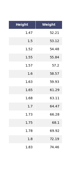
To get started with the simple regression, we use this small dataset from wikipedia describing the average heights and weights for American women aged 30–39.

As this sample has been used previously in statistic analytics, we take for granted that the sample is representative of the population (all American women aged 30-39). However, this sample is very small and normally we should always check that the sample is in line with the population to avoid a biased dataset.

#The variables are height in meters and weight in kilograms.
Height = [1.47, 1.50, 1.52, 1.55, 1.57, 1.60, 1.63, 1.65, 1.68, 1.70, 1.73, 1.75, 1.78, 1.80, 1.83]
Weight = [52.21, 53.12, 54.48, 55.84, 57.20, 58.57, 59.93, 61.29, 63.11, 64.47, 66.28, 68.10, 69.92, 72.19, 74.46]


#Create a dataframe
dfH_W = pd.DataFrame({'Height':Height,'Weight':Weight})


dfH_W

Observations

We can clearly see that both the variables are continous variables, as they are measured, not counted. If both height and weight were defined in intervals, like in integers only, then they would be discrete. However, most people are not exactly 1.70 or 1.60, they tend to be something more granular.

#Lets plot the variables
plt.scatter(dfH_W["Height"], dfH_W["Weight"])
plt.ylabel('Weight')
plt.xlabel('Height')
plt.title("meters vs kilograms")
plt.show()

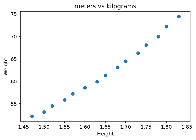
From the scatter plot there seem to be a correlation between height and weight.

Let’s get the values we need:

y = dfH_W["Weight"].values
X = dfH_W["Height"].values

#Add the ones, so we can estimate the intercept

X = np.vstack((np.ones(len(X)), X)).T

We can now implement the estimate of the least square parameter as we derived above:

$$ b = (X^TX)^{-1}X^Ty $$

b = np.linalg.inv(X.T.dot(X)).dot(X.T).dot(y)

The output of b is the intercept followed by the parameter for x (height), which gives us the smallest error term and hence the best fit

array([-39.06195592,  61.27218654])

To get the estimated y; $\hat{y}$: $$ \hat{y} = Xb $$

yhat = X.dot(b)

#Let us plot the least square line:
plt.scatter(dfH_W["Height"], dfH_W["Weight"])
#Select second column of X.
plt.plot(X[:,1], yhat, color = 'pink')
plt.ylabel('Weight')
plt.xlabel('Height')
plt.title("meters vs kilograms")
plt.show()

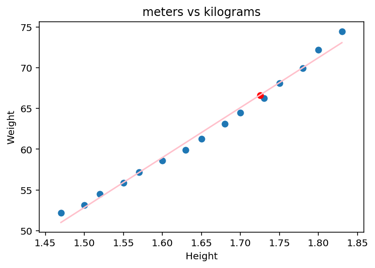
The least square line seems like a good fit for the sample data.

From this we could also make an estimate of weight based on your height if you are an American woman between 30-39:

#Lets say you are 1.725
y_est = b[0] + b[1]*1.725

Let us plot it:

plt.scatter(dfH_W["Height"], dfH_W["Weight"])
plt.scatter(1.725, y_est, color = 'red')
#Select second column of X.
plt.plot(X[:,1], yhat, color = 'pink')
plt.ylabel('Weight')
plt.xlabel('Height')
plt.title("meters vs kilograms")
plt.show()

Assumptions

Great, so we managed to derive the least square and got our estimate. But now we have to check that all the assumptions of the ordinary least square are holding up.

Let us plot the residuals to see if they are random

plt.plot((y-yhat), 'o', color = 'darkblue')
plt.title('Residual plot')
plt.xlabel('Independent variable')
plt.ylabel('Residual')
plt.show

<function matplotlib.pyplot.show(*args, **kw)>

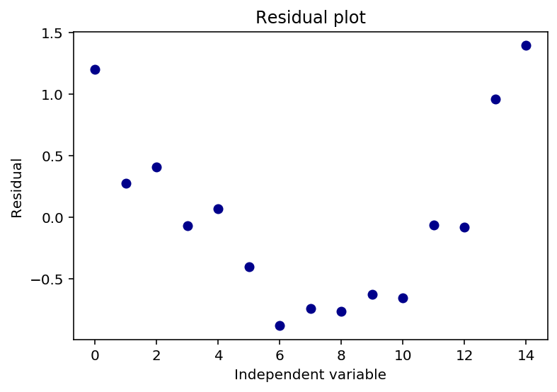
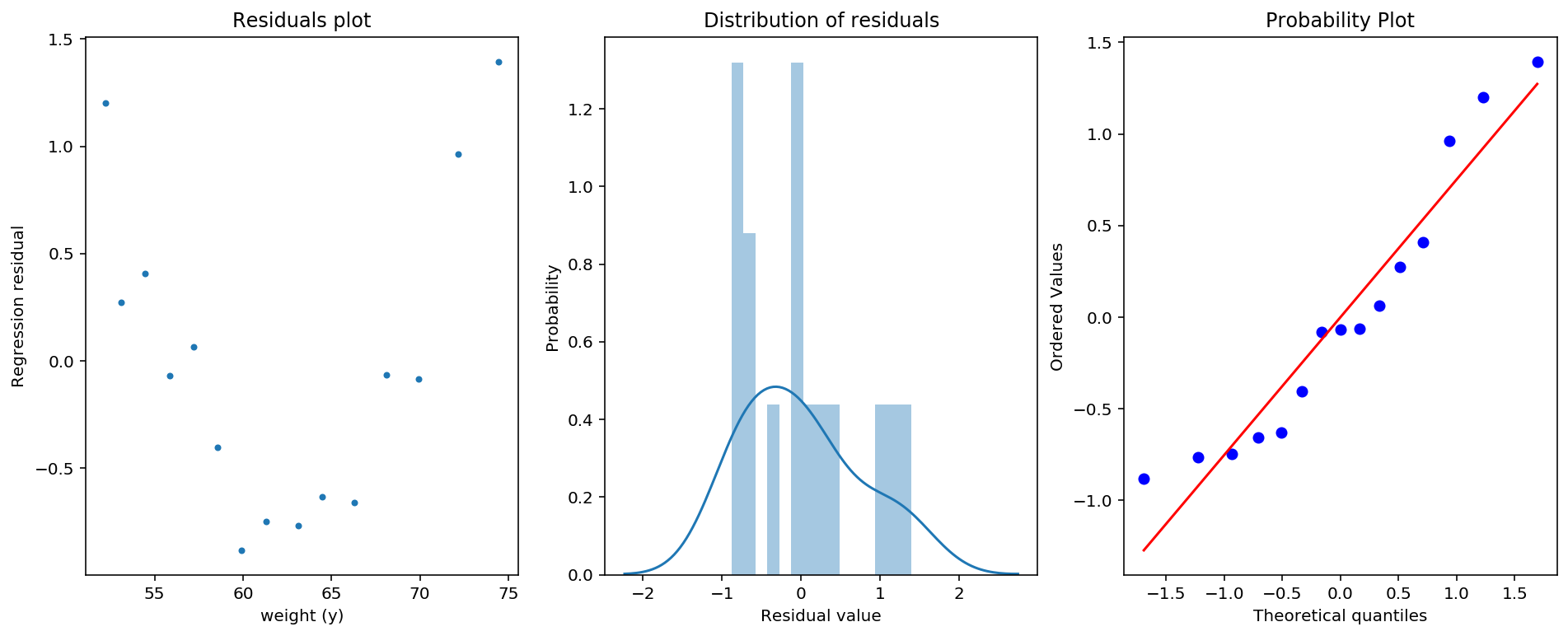
The above plot of the residuals shows a u-shaped pattern, which does speak for that the data is nonlinear.

I will not delwe in to this now, but we could possibly transform one of the variables.

However, as we will see later, the $R^2$ and the $ \bar{R}^2 $ shows that the model describe the data quite well, but to be clear, we should not be too focused on the $R^2$ and the $ \bar{R}^2 $.

Homoskedasticity & Normality

From the graphs under there is clearly something going on with the residual plot, and we can interpret that we are not dealing with homoskedastic errors, rather heteroskedastic. The distribution of the residuals is also not entirely normal, and the probability plot shows that we gave fat tails. Much if this we can assign to the tiny sample we have. So if we would increase our sample, we could rely on law of large numbers and central limit theorem to get appropriate measurments.

To check for normality we could perform would be the Jarque-Bera or the Sharpio-Wilk to test. To check for heteroskedasticity we could use the Breusch-Pagan test.

If it does not help to get more data, we would consider using robust standard errors to deal with this. Like White robust standard errors. But we will not focus on this for now.

fig, (ax1, ax2, ax3) = plt.subplots(1,3, figsize = (16,6))

#Figure 1: residual plot
ax1.plot(y,(y-yhat), marker = '.', linestyle = 'none')
ax1.set_xlabel('weight (y)')
ax1.set_ylabel('Regression residual')
ax1.set_title('Residuals plot')

#Figure 2: Plot of the distribution of the residuals
ax2 = sns.distplot(y-yhat,ax = ax2, bins = 15)
ax2.set_ylabel('Probability')
ax2.set_xlabel('Residual value')
ax2.set_title('Distribution of residuals')

#Figure 3: QQ plot comparing residual quantiles to theoretical normal quantiles
ax3 = stats.probplot(y-yhat, dist = "norm", plot = plt)
plt.show()

$R^2$

To see how well our model fits the data, we can find the sum of squared residuals (SSR) and divide it by the total sum of squares (SST), which we call the $R^2$.

$$ R^2 = 1 - \frac{SSR}{SST} = 1 - \frac{\Sigma^n_{t=1}(y_{t}-\hat{y_{t}})^2}{\Sigma^n_{t=1}(y_{t}-\bar{y_{t}})^2} $$

$R^2$ is the fraction of the variance in y that the model explains
SSE is the sum of squares which are explained by the regression model
SSR is the sum of squared errors the model does not explain
SST is the sum of SSR and SSE

#Caluclations done in matrix format.
SSR = np.dot((y-yhat).T,y-yhat)
SSE = np.dot(yhat - np.mean(yhat),yhat - np.mean(yhat))
SST = np.dot(y - np.mean(yhat),y - np.mean(yhat))

Rsquared = 1 - (SSR / SST)
Rsquared

0.9891969224457968

$\bar{R}^2$

From the $R^2$, we can see that the fit of the model is very good.

A problem is that for larger models (more independent variables), you will always increase $R^2$ when adding an additional independent variable.

Therefore we can use the adjusted $R^2$:

$$ \bar{R}^2 = 1 - (1 - R^2) \frac{n-1}{n-p-1}$$

Where $p$ is the number of parameters excluding the intercept, and $n$ is the number of observations.

adjustedR = 1 - (1 - Rsquared)*(len(X)-1)/(len(X)-1-1)
adjustedR

0.9883659164800889

$Standard$ $error$ $(s)$

We can also look at the standard error of the sample to try to find the godness of fit.

There are many different ways of expressing this, but most commonly used is $s$, $\hat{\sigma}$ and sometimes MSE. We will use $s$ as it clearly explains the sigma for the sample, while $\sigma$ is many times used for the population sigma. They all to some extent describe the sum of squared residuals divided on n adjusted for the degrees of freedom.

$$ MSE = s = \hat{\sigma} = \sqrt{\frac{\Sigma(y-\hat{y})^2}{N-p}}$$

Where p is the number of parameters including intercept.

#Variance of the sample
vs = (SSR)/(len(X)-2)

#Standard error of the sample
s = np.sqrt(vs)
s

0.7590762809485361

To get the standard error of the parameters $\beta_{0},\beta_{1}$, we use this formula:

$$ variance(\beta) = s^2(X^TX)^{-1}$$

Where the symmetric matrix in this case represent:

$$ variance(\beta) = \begin{pmatrix} Var(b_{0}|x) & Cov(b_{0},b_{1}|x) \ Cov(b_{0},b_{1}|x) & Var(b_{1}|x) \end{pmatrix} $$

var_beta = np.diag(np.dot(s**2,np.linalg.inv(np.dot(X.T,X))))
var_beta

array([8.63185027, 3.15390162])

We extract the variance of the covariance matrix and square it. The nice thing is that the OLS method assumes no correlation in the error terms, and thus we only care about the diagonal elements, the variance which gives us the standard error.

se_beta = np.sqrt(var_beta)
se_beta

array([2.93800107, 1.77592275])

Hypothesis testing

T-test

We can now check if the parameters are significant using a table or functions in python.

$H_{0}$ for both parameters independently: $\beta_{0}$, $\beta_{1}$ $=0$

$H_{1}$ for both parameters independently: $\beta_{0}$, $\beta_{1}$ $\neq 0$

We check if the two parameters are significant with a t-test:

$$t_{b_{0}} = \frac{b_{0}}{S_{b_{0}}}$$

$$t_{b_{1}} = \frac{b_{1}}{S_{b_{1}}}$$

t_val = b/se_beta
t_val

array([-13.29541924,  34.5016057 ])

We get the corresponding p values of the two parameters, and we can clearly see that they are significant by a good margin, and we discharge the $H_{0}$

#We multiply by 2 to get both tails
pval_b = (1 - stats.t.cdf(abs(t_val), len(X) -2) ) * 2
pval_b

array([6.05490014e-09, 3.59712260e-14])

F-test

F-test is a special case of the wald-test So far we have only tested the parameters independently, but we can also use the f-test to test for:

$H_{0}$ for both parameters jointly: $\beta_{0} = \beta_{1} = 0$

$H_{1}$ for both parameters jointly: $\beta_{0} \neq \beta_{1} \neq 0$

as in the t-test, we can clearly see the f-test is significant and we discharge $H_{0}$

#F-statistics
F = SSE / vs

#P-value
F_pval = (1 - stats.f.cdf(F, 1, len(X) -2 ) )

F, F_pval

(1190.3607955486298, 3.608224830031759e-14)

Condfidence Interval

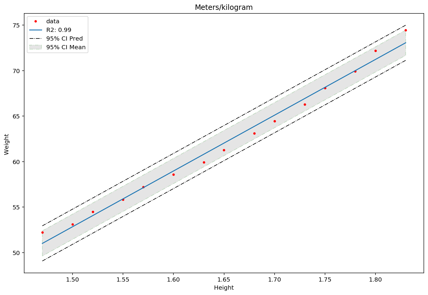
To finish of with the simple linear regression, we get the confidence intervals and plot them.

We get the t-statistics and the confidence intervals, where we want to be confident up to the 95 percentile (using the percent point function (PPF) from scikit stats package). As we are using the sample standard error and not the population standard error, we use the student-t distribution (It has a fatter tail than the normal distribution).

t = stats.t.ppf(.95,len(X) - 2)
#We calculate leverage. Leverage is a point which has unormally high independet variable value.
#While an outlier has an unormally high y value (relative to the fitted line)
h = (1 / len(X)) + (dfH_W["Height"] - np.mean(dfH_W["Height"]))**2 / ((dfH_W["Height"] - np.mean(dfH_W["Height"]))**2)
ConfInt_up = b[0] + b[1] * dfH_W["Height"] + t * np.sqrt(vs * h)
ConfInt_down = b[0] + b[1] * dfH_W["Height"] - t * np.sqrt(vs * h)
ConfPred_up = b[0] + b[1] * dfH_W["Height"] + t * np.sqrt(vs * (1 + h))
ConfPred_down = b[0] + b[1] * dfH_W["Height"] - t * np.sqrt(vs * (1 + h))

#Plot the x and y values in a scatter
plt.figure(figsize = (12,8))
plt.plot(dfH_W["Height"], y, marker = '.', linestyle = 'none', label = 'data', color="red")
plt.xlabel('Height')
plt.ylabel('Weight ')
plt.title('Meters/kilogram')

#Make regression line to plot
x_vals = np.array([min(dfH_W["Height"]),max(dfH_W["Height"])])
y_vals = b[0] + x_vals * b[1]
plt.plot(x_vals,y_vals, label = 'R2: %0.2f '%(Rsquared))

#Plot the Confidence Intervals
plt.fill_between(sorted(dfH_W["Height"]), sorted(ConfInt_up), sorted(ConfInt_down), alpha = .2, facecolor='grey', linestyle='dashdot', edgecolor = 'green', label = '95% CI Mean'  )
plt.plot(sorted(dfH_W["Height"]), sorted(ConfPred_up), linewidth=1, linestyle='dashdot', color = 'black')
plt.plot(sorted(dfH_W["Height"]), sorted(ConfPred_down), linewidth=1, linestyle='dashdot', color = 'black', label = '95% CI Pred')

plt.legend()
plt.show()

Outputs

Key_output_single = pd.DataFrame({'Degrees of Freedom':[X.shape[1], len(X) - X.shape[1] -1, len(X)-1], 
              'Sum of Squares':[SSE,SSR,SST],
              'Mean Square': [SSE / X.shape[1], SSR / (len(X)- X.shape[1] -1),''], 
              'F Value': [F,'',''], 'Pr > F': [F_pval,'',''], 
              'Dependent Mean': [np.mean(yhat),'',''],
              'R Squared':[Rsquared,'',''],'Adj R Squared':[adjustedR,'','']}, ['Model','Errors','Total'])


Param_output_single = pd.DataFrame({'Coefficients':b,'Standard Errors': se_beta,'t-values': t_val, 
              'Pr > |t|': pval_b}, 
             ['intercept','Height'])

Key_output_single

	Degrees of Freedom	Sum of Squares	Mean Square	F Value	Pr > F	Dependent Mean	R Squared	Adj R Squared
Model	2	685.882082	342.941	1190.36	3.60822e-14	62.078	0.989197	0.988366
Errors	12	7.490558	0.624213
Total	14	693.372640

Param_output_single

Coefficients	Standard Errors	t-values	Pr > \|t\|
-39.061956	2.938001	-13.295419	6.054900e-09
61.272187	1.775923	34.501606	3.597123e-14

Intermediate conclusion

In general from the analysis we have done, the sample is very small, and therefore it is advisable to collect more data before doing further analysis.

Luckily, when we have taken this road using matrices, it is a very straight forward procedure to add more independent variables, to get extra dimensions to what you want to infer. What you will have to take in to considertion is that you will have less degrees of freedom when you add more independent (exploratory) variables.

In the simple regression we usually deducted two degrees of freedom; the intercept and the slope parameters, from the total number of observations, while for a multivariate regression, we need to subtract more degrees of freedom, since you are penalized by adding more independent variables.

So lets have a go at a multiple regression, reusing what we have done so far. I will not dive in to data exploration, but if you want, there is a good exploratory anaylsis of the data set used here.

Multivariate Regression

multidf = pd.read_fwf("auto-mpg.data", names = ['mpg','cylinders','displacement',
                     'horsepower','weight','acceleration', 'model_year', 'origin', 'car_name'], index_col="car_name")

#Remove na values and set horsepower from object to float
multidf = multidf[multidf['horsepower'].map(lambda x: str(x)!="?")]
multidf['horsepower'] = multidf['horsepower'].astype('float')
multidf

mpg	cylinders	displacement	horsepower	weight	acceleration	model_year	origin	car_name
18.0	8	307.0	130.0	3504.0	12.0	70	1	chevrolet chevelle malibu
15.0	8	350.0	165.0	3693.0	11.5	70	1	buick skylark 320
18.0	8	318.0	150.0	3436.0	11.0	70	1	plymouth satellite
16.0	8	304.0	150.0	3433.0	12.0	70	1	amc rebel sst
17.0	8	302.0	140.0	3449.0	10.5	70	1	ford torino

A quick summary of the dataset:

1. mpg:           continuous
2. cylinders:     multi-valued discrete
3. displacement:  continuous
4. horsepower:    continuous
5. weight:        continuous
6. acceleration:  continuous
7. model year:    multi-valued discrete
8. origin:        multi-valued discrete
9. car name:      string (unique for each instance) (made index)

#Get values of y and X
y_m = multidf["mpg"].values
X_m = multidf.iloc[:,1:].values

#Add the ones to X, so we can estimate the intercept

X_m = np.append(np.ones([X_m.shape[0],  1], dtype=np.int32),X_m, axis=1)

Get Parameters

b_m = np.linalg.inv(X_m.T.dot(X_m)).dot(X_m.T).dot(y_m)

Get $\hat{y}$

yhat_m = X_m.dot(b_m)

$R^2$

#Caluclations done in matrix format.
SSR_m = np.dot((y_m-yhat_m).T,y_m-yhat_m)
SSE_m = np.dot(yhat_m - np.mean(yhat_m),yhat_m - np.mean(yhat_m))
SST_m = np.dot(y_m - np.mean(yhat_m),y_m - np.mean(yhat_m))

Rsquared_m = 1 - (SSR_m / SST_m)

$\bar{R^2}$

adjustedR_m = 1 - (1 - Rsquared_m)*(len(multidf)-1)/(len(multidf)-len(multidf.columns)-1)

$Standard$ $error$ $(s)$

#Variance of the sample
vs_m = (SSR_m)/(len(multidf)-len(multidf.columns))

#Standard error of the sample
s_m = np.sqrt(vs_m)

Hypothesis testing

T-test

#Get the variance of the betas, using np.diagonal of the 8x8 matrix
var_b_m = np.diag(np.dot(s_m**2,np.linalg.inv(np.dot(X_m.T,X_m))))

#square root of variance to get standard errors
s_b_m = np.sqrt(var_b_m)

#T-values
t_values = b_m/ s_b_m
#p-values
p_values = (1 - stats.t.cdf(abs(t_values), len(multidf) -len(multidf.columns)) ) * 2

F-test

#F-statistics
F_value = (SSE_m / len(multidf.columns)) / (SSR_m / (len(multidf) - len(multidf.columns) -1))

#P-value
F_pvalue = (1 - stats.f.cdf(F, len(multidf.columns), len(multidf) -len(multidf.columns)-1 ) )

Additional tests

As I have been pretty brief in explaning the multivariate regression, and because of the problem of plotting a multidimensional regression for inference, I have thrown in some tests that can be done to check if the assumptions we talked about earlier holds.

Multicolinearity (VIF-test & Tolerance test)

We create a loop where we delete one independent variable (column) from the X matrix and use that independent variable as the dependent variable (y). We then run the regression until we get R2 as we did above. In the end we calculate the VIF and Tolerance score and append it to the list.

Formula: $$Tol(x_{p}) = 1 - R^2_{p}$$

$$VIF(x_{p}) = \frac{1}{Tol(x_{p})} = \frac{1}{1 - R^2_{p}}$$

If: $ Tol < 0.5 $ and/or $VIF > 2$ we need to check for multicolinearity.

Where p is number of parameters not including the intercept

VIF = ['']
Tol = ['']

#We start from index 1 to not include intercept
for i in range(1,X_m.shape[1]):
    tmp_X = np.delete(X_m, i, 1)
    tmp_y = X_m[:,i]
    tmp_b = np.linalg.inv(tmp_X.T.dot(tmp_X)).dot(tmp_X.T).dot(tmp_y)
    tmp_yhat = tmp_X.dot(tmp_b)
    tmp_SSR = np.dot((tmp_y-tmp_yhat).T,tmp_y-tmp_yhat)
    tmp_SST = np.dot(tmp_y - np.mean(tmp_yhat),tmp_y - np.mean(tmp_yhat))
    tmp_R2 = 1 - (tmp_SSR / tmp_SST)
    VIF.append(1/(1-tmp_R2))
    Tol.append(1 - tmp_R2)

Skewness & Kurtosis

Skewness is a measure of asymmetry of the distribution, while kurtosis is a measure of its curvature.

If we have high kurtosis the tails tend to be fat, and if we have skewness in any direction, the mode and the mean are not the same.

#Get absolute errors
A_e = y_m - yhat_m

Skew = np.mean(A_e**3.0 ) / np.mean( A_e**2.0 )**(3.0/2.0)
Kurtosis = np.mean( A_e**4.0 ) / np.mean( A_e**2.0 )**(4.0/2.0)

Autocorrelation (Durbin-Watson)

DW = np.sum( np.diff( A_e )**2.0 ) / SSR_m

Normality (Jarque-Bera test)

JB_test = (len(X_m)/6.0) * ( Skew**2.0 + (1.0/4.0)*( Kurtosis - 3.0 )**2.0 )
JB_p = 1.0 - stats.chi2(2).cdf(JB_test)

Heteroskedasticity (White test)

#Square the error terms calculated above
u_squared = A_e**2

#stack yhat and yhat squared in a matrix
#An easier approach than to regress over all independent variables and their interactions, 
#which grows increasingly large the more independent variables you have
x_mat = np.column_stack((yhat_m,yhat_m**2))
x_mat = np.append(np.ones([x_mat.shape[0],  1], dtype=np.int32),x_mat, axis=1)
delta_m = np.linalg.inv(x_mat.T.dot(x_mat)).dot(x_mat.T).dot(u_squared)

yhat_mat = x_mat.dot(delta_m)


SSR_mat = np.dot((u_squared-yhat_mat).T,u_squared-yhat_mat)
SSE_mat = np.dot(yhat_mat - np.mean(yhat_mat),yhat_mat - np.mean(yhat_mat))



#F-statistics
F_value_mat = (SSE_mat / X_m.shape[1]) / (SSR_mat / (len(x_mat) - X_m.shape[1] -1))

#P-value
F_pvalue_mat = (1 - stats.f.cdf(F, x_mat.shape[1], len(x_mat) -X_m.shape[1]-1 ) )

Outputs

Key_output = pd.DataFrame({'Degrees of Freedom':[len(multidf.columns), len(X_m) - len(multidf.columns) -1, len(X_m)-1], 
              'Sum of Squares':[SSE_m,SSR_m,SST_m],
              'Mean Square': [SSE / len(multidf.columns), SSR_m / (len(X_m)- len(multidf.columns) -1),''], 
              'F Value': [F_value,'',''], 'Pr > F': [F_pvalue,'',''], 
              'Dependent Mean': [np.mean(yhat_m),'',''],
              'R Squared':[Rsquared_m,'',''],'Adj R Squared':[adjustedR_m,'',''],
              'Skew':[Skew,'',''],'Kurtosis':[Kurtosis,'',''],
              'DW':[DW,'',''],
              'JB Value':[JB_test,'',''],'Pr > JB':[JB_p,'',''],
              'White F value':[F_value_mat,'',''],'White  Pr > F':[F_pvalue_mat,'','']}, ['Model','Errors','Total'])


Param_output = pd.DataFrame({'Coefficients':b_m,'Standard Errors': s_b_m,'t-values': t_values, 
              'Pr > |t|': p_values,'Tolerance': Tol, 'VIF': VIF}, 
             ['intercept','cylinders','displacement','horsepower','weight','acceleration', 'model_year', 'origin'])

Key_output

	Degrees of Freedom	Sum of Squares	Mean Square	F Value	Pr > F	Dependent Mean	R Squared	Adj R Squared	Skew	Kurtosis	DW	JB Value	Pr > JB	White F value
8	19566.780939	85.7353	220.299	1.11022e-16	23.4459	0.821478	0.817749	0.52909	4.4599	1.30925	53.1005	2.94698e-12	2.98955	1.11022e-16
383	4252.212530	11.1024
391	23818.993469

Thoughts

From the sum of squares, we can see the model is explaining the data well
We reject H0 that the parameters are all 0
Both R squared and adjusted R squared tell us the godness of fit is not too bad
The skewness shows the distribution is approximately symmetric, there seems to be som fat tails in the distribution, but the Jarque-Bera test tells us to reject H0 and the distribution is approximately normal
The Durbin-Watson test shows that there is some positive autocorrelation
The White test has rejected the H0, and we do not seem to have any heteroskedasticity

Param_output

Coefficients	Standard Errors	t-values	Pr > \|t\|	Tolerance	VIF
-17.218435	4.644294	-3.707438	2.401841e-04
-0.493376	0.323282	-1.526147	1.277965e-01	0.0931312	10.7375
0.019896	0.007515	2.647430	8.444649e-03	0.0457943	21.8368
-0.016951	0.013787	-1.229512	2.196328e-01	0.100566	9.94369
-0.006474	0.000652	-9.928787	0.000000e+00	0.0923254	10.8313
0.080576	0.098845	0.815174	4.154780e-01	0.380835	2.62581
0.750773	0.050973	14.728795	0.000000e+00	0.803244	1.24495
1.426140	0.278136	5.127492	4.665681e-07	0.564211	1.77239

Thoughts:

The intercept has a significant large impact on the dependent variable
Horsepower, Cylinders and Acceleration are not significant, so we keep H0 for these parameters.
Displacement seems to be affected by multicolineariy, but good to look at cylinder and weight.
To deal with multicollinearity we could use a stepwise to remove variables one at the time to see if our estimates are getting better. If not we could use a penalizer, like what we will look at further down

Generalized Least Square

If there is heteroskedasticity or autocorrelation or both present in the OLS, a good way to deal with this is to use the Generalized Least Square (GLS). However, in most cases there is no strong theory of how the heteroskedasticity should look like, so it is more common among especially econometricians to opt for robust standard errors, as an easier way out.

As we do not possess the true covariance matrix, we will rather have to work with the feasable GLS (fGLS), which in this case will be the Weighted Least Square (WLS).

The model will not be Best Linear Unbiased Estimate (BLUE), as it will be biased, but we can take comfort in that it has a tendency to be asymptotically unbiased when the sample size goes to infinity.

When we have heteroskedasticity in the error terms, we know that the error terms are not constant through the observations, they will have different variance.

$$Var(\epsilon|X) \neq \sigma^2$$

Below you find the parameters derived given we have heteroskedasticity. To see how we get to this result have a look at this link.

$$ \hat{\beta}_{FGLS} = (X^T{\hat{\Omega}}^{-1}X)^{-1}X^T{\hat{\Omega}}^{-1}y$$

To estimate the equation we find the variance of the standard error given the independent variables and the variance we got from the OLS regression: As given by woolridge:

$$ var(u^2|X) = u^2 = \sigma^2 \exp(\delta_{0} + \delta_{1}x_{1} + \delta_{2}x_{2} + …. + + \delta_{n}x_{n})$$

The reason why we use the exponent is because nothing is stopping the variance in a linear relationship to be negative.

The reason why the standard error is squared is because we know the second term is 0:

$$var(u^2|X) = E[u_{i}^2|X]-[E[u_{i}|X]]^2$$

As we are dealing with a sample we use $\hat{u}^2$ instead of $u^2$, and we already know this value from the multivariate regression from eariler. By taking the log of both sides, we get:

$$log(\hat{u}^2) = \delta_{0} + \delta_{1}x_{1} + \delta_{2}x_{2} + …. + + \delta_{n}x_{n} + e$$

The predicted value is then:

$$\hat{g}_{i} = \hat{\delta}_{0} + \hat{\delta}_{1}x_{1} + \hat{\delta}_{2}x_{2} + …. + + \hat{\delta}_{n}x_{n} + \hat{e}$$

We then get the variance on its own:

$$\hat{h}_{i} = \exp(\hat{g}_{i}) = \exp\hat{(\log(\hat{u}^2))} = \hat{\hat{u}^2} $$

So to summarize we do:

$$ \frac{y_{i}}{\sqrt{\hat{h}_{i}}} = \frac{\hat{\beta}}{\sqrt{\hat{h}_{i}}} + \frac{\hat{\beta}_{i}x_{i}}{\sqrt{\hat{h}_{i}}} + \frac{{\epsilon}_{i}}{\sqrt{\hat{h}_{i}}}$$

We will stick to the same dataset as in the multivariate, even though it does not show any heteroskedasticity, just for simplicity. But feel free to implement it with another dataset that truly shows heteroskedasticity:

#Lets get the error we found in the section of skewness and kurtosis
#We square it and take the log:
ee_sq = np.log(A_e**2)

#run the regression:
deltas = np.linalg.inv(X_m.T.dot(X_m)).dot(X_m.T).dot(ee_sq)
#Get g_hat
g_hat = X_m.dot(deltas)

#Get h_hat
h_hat = np.exp(g_hat)

#Divide by 1 and take the square root of h_hat
h_hat_sq = np.sqrt(h_hat)

#We find the parameters which should be homoskedastic
fgls = np.linalg.inv((X_m.T/h_hat_sq).dot(X_m)).dot((X_m.T/h_hat_sq)).dot(y_m)

#Get y_hat prediction
y_hat_homo = X_m.dot(fgls)

Feel free to implement the tests from the multivariate OLS.

Robust Standard Errors (White standard errors)

To not take the route around the fgls, we could as we talked about earlier get robust standard errors. As this is a trivial task, I will show how to do it before we move on to ridge regression. We will use the data from the mulivariate regression:

We know from earlier that the variance of the OLS is: $$ variance(\beta) = s^2(X^TX)^{-1}$$

However when the assumption is violated, we get: $$V[\hat{\beta}_{OLS}] = V[(X^TX)^{-1}X^Ty] = (X^TX)^{-1}X^T\Sigma X(X^TX)^{-1}$$ $$where$$ $$ \Sigma = V[u]$$

if errors are independent, but have individual variance, then: $$ V[\hat{\beta}] = (X^TX)^{-1}X^T diag(\hat{u_{1}^2},…,\hat{u}_{n}^2) X(X^TX)^{-1}$$

#Import the residuals from above
resi = A_e

#Find the heteroskedastic consistent variance covariance matrix
vcov_h_consistent = np.linalg.inv(X_m.T.dot(X_m)).dot(X_m.T).dot(np.diag(resi**2)).dot(X_m).dot(np.linalg.inv(X_m.T.dot(X_m)))
#Get square root of the diagonal elements in the covariance matrix and voila you have robust standard errors.
e_h_consistent = np.sqrt(np.diag(X_m.dot(vcov_h_consistent).dot(X_m.T)))

From here on you could implement these robust standard errors in your analysis of the multivariate case, implementing all the tests as we normally did.

Ridge Regression

To deal with multicollinearity and large variance which can be far from “actual value”, we can use the Ridge regression. The goal is to reduce the standard error by adding some bias.

In general it is a normal regression with a $L_{2}$ regularization (Euclidean norm (The shortest distance from one point to another). You know from earlier in the simple regression we got:

$$S(b) = (y-Xb)^T(y-Xb)$$

What the Ridge regression does, is to add a regularizer $\lambda$

$$\hat{b}_{R} = (y-Xb)^T(y-Xb)+\lambda b^Tb$$ Or in machine learning terms: $$ \hat{b}_{R} = ||y-Xb||^2_{2}+\lambda ||b||^2_{2} $$

The derivation of the equation is very similar to what we did for the simple regression, but we end up with this equation after deriving it:

$$ \hat{b}_{R} = (X^TX + \lambda I)^{-1}X^Ty $$

The cool thing about this type of regression with a regulizer, is that we can iterate through the different values of $\lambda$ to find the $\lambda$ that minimizes the regression, getting us the least square.

As you will see in the code, it is important to standardize both the dependent and independet variables before performing the regression. This is also something to have in mind when performing any regression. Standardization happens through subtracting the mean and dividing by the standard error.

Also be sure to take note, that if you should want to get the rest of the statistics for the parameters, sum of squares and so on, you need to subtract one extra degree of freedom, as the $\lambda$ parameter is in the ridge regression

#Standardize the data:
X_mS = (X_m[:,1:] - np.mean(X_m[:,1:])) / np.std(X_m[:,1:])
y_mS = (y_m - np.mean(y_m)) / np.std(y_m)

#By not standardizing the coefficients we can see that with lambda = 0, 
#we get the same values as with the mulitvariate regression, using X and y below instead:
#X_mS = X_m[:,1:]
#y_mS = y_m

#Add the ones for intercept
X_mS = np.append(np.ones([X_m.shape[0],  1], dtype=np.int32),X_mS, axis=1)

#Get the identity matrix
I = np.identity(X_mS.shape[1])

#The lambda parameter for tuning
alpha = 0.0000001

#The ridge regression
ridge_reg = np.linalg.inv((X_mS.T.dot(X_mS)) + alpha * I).dot(X_mS.T).dot(y_mS)

#Get the yhat
y_hat_R = X_mS.dot(ridge_reg)

#Caluclations done in matrix format.
SSR_m_R = np.dot((y_mS-y_hat_R).T,y_mS-y_hat_R)
SSE_m_R = np.dot(y_hat_R - np.mean(y_hat_R),y_hat_R - np.mean(y_hat_R))
SST_m_R = np.dot(y_mS - np.mean(y_hat_R),y_mS - np.mean(y_hat_R))

Rsquared_m = 1 - (SSR_m_R / SST_m_R)
Rsquared_m

0.821478063939711

What we can interpret from the results of the R squared is that the closer the hyperparamter $\lambda$ is to 0, the higher the value of R squared, even though R squared does not tell the whole picture. And as we remember from earlier, that when $\lambda$ is zero, it is just like a standard ols.

As an extra I have added an approach where we try to check different values of lambda and iterate through the MSE to find the lambda and MSE that minimize the loss.

Let’s us divide the dataset from above for MPG in to a train and test set. We create a function and then test the ridge regression on the test set.

X_train, X_test, y_train, y_test = train_test_split(X_mS, y_mS, test_size=0.1)



class Ridge_R(object):
    def __init__(self, l_mbda=0.1):
        self.l_mbda = l_mbda
        self.Id = np.identity(X_mS.shape[1])

    def fit(self, X_mS, y_mS):
        self.b = ridge_reg = np.linalg.inv((X_mS.T.dot(X_mS)) + l_ambda * self.Id).dot(X_mS.T).dot(y_mS)

    def predict(self, X_mS):
        return X_mS.dot(self.b)

    def get_params(self, deep=True):
        return {"l_mbda": self.l_mbda}

    def set_params(self, l_mbda=0.1):
        self.l_mbda = l_mbda
        return self

ridge_Reg = Ridge_R()
params = [{"l_mbda": 2.5**np.arange(-5, 10)}]
grid = GridSearchCV(ridge_Reg, params, scoring="neg_mean_squared_error", cv=5, n_jobs=-1, verbose=0)
grid.fit(X_train, y_train)

y_hat_Rc = grid.predict(X_test)
ridge_error = mean_absolute_error(y_test, y_hat_Rc)

/opt/conda/lib/python3.7/site-packages/sklearn/model_selection/_search.py:814: DeprecationWarning: The default of the `iid` parameter will change from True to False in version 0.22 and will be removed in 0.24. This will change numeric results when test-set sizes are unequal.
  DeprecationWarning)

alphas = 2.0**np.arange(-5, 20)
coefs = []
for a in alphas:
    ridge = np.linalg.inv((X_mS.T.dot(X_mS)) + a * np.eye(X_mS.shape[1])).dot(X_mS.T).dot(y_mS)
    y_hatR = X_mS.dot(ridge)
    coefs.append(ridge)

ax = plt.gca()
ax.plot(alphas, coefs)
ax.set_xscale('log')
plt.xlabel('alpha')
plt.ylabel('weights')
plt.title('Ridge coefficients as a function of the regularization')
plt.axis('tight')
plt.show()

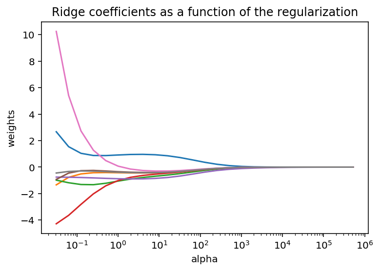
It is quite interesting to see that when we increase the the $\lambda$, the weight (value) of the beta coefficients tends toward zero.

Lasso Regression & Elastic Net

The Lasso regression is very similar to the Ridge regression, but we use the $L_{1}$ norm (taxicab norm) instead, which is the sum of the absolute values of the coefficients. An advantage of using lasso regression is that it has the possibility to null out non important coefficients, and thus null out the independent variables which are not contributing to the output. However, the ridge has an advantage in that the coefficients stay normally distributed.

Therefore we have in machine learning terms: $$ \hat{b}_{R} = ||y-Xb||^2+\lambda ||b||_{1} $$

There does not really exist a good analytical approach to solve the Lasso, since we cannot write out an explicit anaytical form. Taylor B. Arnold at Yale, provides a very good explanation of how to solve the Lasso regression.

The same holds true for Elastic Net, as it confounds both the $L_{1}$ and $L_{2}$ norms.

So as we are focusing on the closed form solutions and in that sense solving with matrices, we leave the iterative approach with gradient decents and such for another posts.

Conclusion:

Using matrix operations instead of looping through variables not only use less code, but also less computational power is needed as you can parallelize it. You also increases your understanding by using matrices instead of using the libraries.

We could have clearly gone deeper in the analysis of the linear regression, but the focus was on how to complete it all with matrices instead of using standard libraries.

Also, you might have noticed that I have not normalized any of the variables. The reason for this is that the OLS is an invariant technique where the substantive answer would not change much with normalization. However, when we go into lasso, ridge and elnet regressions we standardized the data.

Lastly, we could have performed all the calculations using functions and classes, as it is more clean, and it makes more sense as you can reuse it later on. However, it might not be so clear to many what we actually are doing then, so I prioritized understanding, not efficiency and cleanness.

A Regression

Types of regressions

Ordinary Least Square Regression (OLS)

Assumptions

Finding the parameters of the linear regression

Let’s get our hands dirty

Observations

Assumptions

Homoskedasticity & Normality

$R^2$

$\bar{R}^2$

$Standard$ $error$ $(s)$

Hypothesis testing

T-test

F-test

Condfidence Interval

Outputs

Intermediate conclusion

Multivariate Regression

Get Parameters

Get $\hat{y}$

$R^2$

$\bar{R^2}$

$Standard$ $error$ $(s)$

Hypothesis testing

T-test

F-test

Additional tests

Multicolinearity (VIF-test & Tolerance test)

Skewness & Kurtosis

Autocorrelation (Durbin-Watson)

Normality (Jarque-Bera test)

Heteroskedasticity (White test)

Outputs

Thoughts

Thoughts:

Generalized Least Square

Robust Standard Errors (White standard errors)

Ridge Regression

Lasso Regression & Elastic Net

Conclusion:

FEATURED TAGS